Benchmarking optimizers

Benchmarking is very important when researching new algorithms or selecting the most approriate ones.

The package SolverBenchmark exports the function bmark_solvers that runs a set of optimizers on a set of problems. JSOSuite.jl specialize this function, see bmark_solvers.

The JuliaSmoothOptimizers organization contains several packages of test problems ready to use for benchmarking. The main ones are

OptimizationProblems.jl: This package provides a collection of optimization problems in JuMP and ADNLPModels syntax;
CUTEst.jl;
NLSProblems.jl.

In this tutorial, we will use OptimizationProblems.jl with automatic differentiation.

Benchmark with OptimizationProblems.jl

using ADNLPModels, OptimizationProblems, JSOSuite

The package OptimizationProblems.jl provides a meta containing all the problem information. It is possible to then select the problems without evaluating them first.

selected_meta = OptimizationProblems.meta
selected_meta = selected_meta[(selected_meta.nvar .< 200), :] # choose problem with <200 variables.
selected_meta = selected_meta[.!selected_meta.has_bounds .&& (selected_meta.ncon .== 0), :]; # unconstrained problems
list = selected_meta[!, :name]

178-element Vector{String}:
 "AMPGO02"
 "AMPGO03"
 "AMPGO04"
 "AMPGO05"
 "AMPGO06"
 "AMPGO07"
 "AMPGO08"
 "AMPGO09"
 "AMPGO10"
 "AMPGO11"
 ⋮
 "srosenbr"
 "thurber"
 "tointgss"
 "tquartic"
 "tridia"
 "vardim"
 "vibrbeam"
 "watson"
 "woods"

Then, we generate the list of problems using ADNLPModel.

ad_problems = [
  OptimizationProblems.ADNLPProblems.eval(Meta.parse(problem))() for problem ∈ list
]
length(ad_problems) # return the number of problems

We now want to select appropriate optimizers using the JSOSuite.optimizers.

using NLPModelsIpopt
selected_optimizers = JSOSuite.optimizers
# optimizers can solve general `nlp` as some are specific to variants (NLS, ...)
selected_optimizers = selected_optimizers[selected_optimizers.can_solve_nlp, :]
selected_optimizers[selected_optimizers.is_available, :] # optimizers available

6×15 DataFrame

Row	name	name_solver	name_parameters	name_pkg	solve_function	is_available	bounds	equalities	inequalities	specialized_nls	can_solve_nlp	nonlinear_obj	nonlinear_con	double_precision_only	highest_derivative
	String	Symbol	Symbol	String	Symbol	Bool	Bool	Bool	Bool	Bool	Bool	Bool	Bool	Bool	Int64
1	LBFGS	LBFGSSolver	LBFGSParameterSet	JSOSolvers.jl	lbfgs	true	false	false	false	false	true	true	true	false	1
2	R2	R2Solver	FOMOParameterSet	JSOSolvers.jl	R2	true	false	false	false	false	true	true	true	false	1
3	TRON	TronSolver	TRONParameterSet	JSOSolvers.jl	tron	true	true	false	false	false	true	true	true	false	2
4	TRUNK	TrunkSolver	TRUNKParameterSet	JSOSolvers.jl	trunk	true	false	false	false	false	true	true	true	false	2
5	IPOPT	IpoptSolver	not_implemented	NLPModelsIpopt.jl	ipopt	true	true	true	true	false	true	true	true	true	2
6	Percival	PercivalSolver	not_implemented	Percival.jl	percival	true	true	true	true	false	true	true	true	false	2

For the purpose of this example, we will consider 3 optimizers.

select = ["IPOPT", "TRUNK", "LBFGS"]

3-element Vector{String}:
 "IPOPT"
 "TRUNK"
 "LBFGS"

Once the problems and optimizers are chosen, the function bmark_solvers runs the benchmark.

using SolverBenchmark
stats = bmark_solvers(ad_problems, select, atol = 1e-3, max_time = 10.0, verbose = 0)

Dict{Symbol, DataFrames.DataFrame} with 3 entries:
  :IPOPT => 178×42 DataFrame…
  :LBFGS => 178×40 DataFrame…
  :TRUNK => 178×40 DataFrame…

Finally, the result can be processed. For instance, we show here performance profiles comparing the elapsed time and the number of evaluations.

first_order(df) = df.status .== :first_order
unbounded(df) = df.status .== :unbounded
solved(df) = first_order(df) .| unbounded(df)
costnames = ["time", "obj + grad + hess"]
costs = [
  df -> .!solved(df) .* Inf .+ df.elapsed_time,
  df -> .!solved(df) .* Inf .+ df.neval_obj .+ df.neval_grad,
]

using Plots, SolverBenchmark
gr()

profile_solvers(stats, costs, costnames)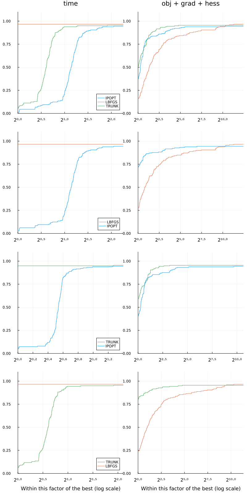

Note that there are fundamental differences between these optimizers as highlighted in the following.

for solver in ["IPOPT", "TRUNK", "LBFGS"]
  println("$solver evaluations:")
  a, b, c, d = eachcol(
    stats[Symbol(solver)][!, [:neval_obj, :neval_grad, :neval_hess, :neval_hprod]]
  )
  println(
    "neval_obj: $(sum(a)),  neval_grad: $(sum(b)), neval_hess: $(sum(c)), neval_hprod: $(sum(d))."
  )
end

IPOPT evaluations:
neval_obj: 99702,  neval_grad: 28720, neval_hess: 28369, neval_hprod: 0.
TRUNK evaluations:
neval_obj: 27366,  neval_grad: 8427, neval_hess: 0, neval_hprod: 115918.
LBFGS evaluations:
neval_obj: 115681,  neval_grad: 86143, neval_hess: 0, neval_hprod: 0.