JSOTutorials.jl

One useful feature of our optimization solvers is the option to add a callback, i.e., a function that is called during the execution of the method, between iterations. It can be used for adding more logging information, for instance to plot the trace of the algorithm, or for having more control over the progress of the method, for instance by adding additional stopping criteria.

---

For these examples, let’s consider a simple extension of the Rosenbrock function:

\[\min\ \sum_{i=1}^N (x_{2i-1} - 1)^2 + (2i)^2 (x_{2i} - x_{2i-1}^2)^2\]

We will implement this in JuMP and use NLPModelsJuMP to bridge the model to our NLPModels format.

using JuMP, NLPModelsJuMP

model = Model()
N = 10
@variable(model, x[1:2N])
@NLobjective(model, Min,
  sum((x[2i - 1] - 1)^2 + (2i)^2 * (x[2i] - x[2i-1]^2)^2 for i = 1:N)
)

nlp = MathOptNLPModel(model)

NLPModelsJuMP.MathOptNLPModel
  Problem name: Generic
   All variables: ████████████████████ 20     All constraints: ⋅⋅⋅⋅⋅⋅⋅⋅⋅⋅⋅⋅⋅⋅⋅⋅⋅⋅⋅⋅ 0     
            free: ████████████████████ 20                free: ⋅⋅⋅⋅⋅⋅⋅⋅⋅⋅⋅⋅⋅⋅⋅⋅⋅⋅⋅⋅ 0     
           lower: ⋅⋅⋅⋅⋅⋅⋅⋅⋅⋅⋅⋅⋅⋅⋅⋅⋅⋅⋅⋅ 0                lower: ⋅⋅⋅⋅⋅⋅⋅⋅⋅⋅⋅⋅⋅⋅⋅⋅⋅⋅⋅⋅ 0     
           upper: ⋅⋅⋅⋅⋅⋅⋅⋅⋅⋅⋅⋅⋅⋅⋅⋅⋅⋅⋅⋅ 0                upper: ⋅⋅⋅⋅⋅⋅⋅⋅⋅⋅⋅⋅⋅⋅⋅⋅⋅⋅⋅⋅ 0     
         low/upp: ⋅⋅⋅⋅⋅⋅⋅⋅⋅⋅⋅⋅⋅⋅⋅⋅⋅⋅⋅⋅ 0              low/upp: ⋅⋅⋅⋅⋅⋅⋅⋅⋅⋅⋅⋅⋅⋅⋅⋅⋅⋅⋅⋅ 0     
           fixed: ⋅⋅⋅⋅⋅⋅⋅⋅⋅⋅⋅⋅⋅⋅⋅⋅⋅⋅⋅⋅ 0                fixed: ⋅⋅⋅⋅⋅⋅⋅⋅⋅⋅⋅⋅⋅⋅⋅⋅⋅⋅⋅⋅ 0     
          infeas: ⋅⋅⋅⋅⋅⋅⋅⋅⋅⋅⋅⋅⋅⋅⋅⋅⋅⋅⋅⋅ 0               infeas: ⋅⋅⋅⋅⋅⋅⋅⋅⋅⋅⋅⋅⋅⋅⋅⋅⋅⋅⋅⋅ 0     
            nnzh: ( 85.71% sparsity)   30              linear: ⋅⋅⋅⋅⋅⋅⋅⋅⋅⋅⋅⋅⋅⋅⋅⋅⋅⋅⋅⋅ 0     
                                                    nonlinear: ⋅⋅⋅⋅⋅⋅⋅⋅⋅⋅⋅⋅⋅⋅⋅⋅⋅⋅⋅⋅ 0     
                                                         nnzj: (------% sparsity)         

  Counters:
             obj: ⋅⋅⋅⋅⋅⋅⋅⋅⋅⋅⋅⋅⋅⋅⋅⋅⋅⋅⋅⋅ 0                 grad: ⋅⋅⋅⋅⋅⋅⋅⋅⋅⋅⋅⋅⋅⋅⋅⋅⋅⋅⋅⋅ 0                 cons: ⋅⋅⋅⋅⋅⋅⋅⋅⋅⋅⋅⋅⋅⋅⋅⋅⋅⋅⋅⋅ 0     
        cons_lin: ⋅⋅⋅⋅⋅⋅⋅⋅⋅⋅⋅⋅⋅⋅⋅⋅⋅⋅⋅⋅ 0             cons_nln: ⋅⋅⋅⋅⋅⋅⋅⋅⋅⋅⋅⋅⋅⋅⋅⋅⋅⋅⋅⋅ 0                 jcon: ⋅⋅⋅⋅⋅⋅⋅⋅⋅⋅⋅⋅⋅⋅⋅⋅⋅⋅⋅⋅ 0     
           jgrad: ⋅⋅⋅⋅⋅⋅⋅⋅⋅⋅⋅⋅⋅⋅⋅⋅⋅⋅⋅⋅ 0                  jac: ⋅⋅⋅⋅⋅⋅⋅⋅⋅⋅⋅⋅⋅⋅⋅⋅⋅⋅⋅⋅ 0              jac_lin: ⋅⋅⋅⋅⋅⋅⋅⋅⋅⋅⋅⋅⋅⋅⋅⋅⋅⋅⋅⋅ 0     
         jac_nln: ⋅⋅⋅⋅⋅⋅⋅⋅⋅⋅⋅⋅⋅⋅⋅⋅⋅⋅⋅⋅ 0                jprod: ⋅⋅⋅⋅⋅⋅⋅⋅⋅⋅⋅⋅⋅⋅⋅⋅⋅⋅⋅⋅ 0            jprod_lin: ⋅⋅⋅⋅⋅⋅⋅⋅⋅⋅⋅⋅⋅⋅⋅⋅⋅⋅⋅⋅ 0     
       jprod_nln: ⋅⋅⋅⋅⋅⋅⋅⋅⋅⋅⋅⋅⋅⋅⋅⋅⋅⋅⋅⋅ 0               jtprod: ⋅⋅⋅⋅⋅⋅⋅⋅⋅⋅⋅⋅⋅⋅⋅⋅⋅⋅⋅⋅ 0           jtprod_lin: ⋅⋅⋅⋅⋅⋅⋅⋅⋅⋅⋅⋅⋅⋅⋅⋅⋅⋅⋅⋅ 0     
      jtprod_nln: ⋅⋅⋅⋅⋅⋅⋅⋅⋅⋅⋅⋅⋅⋅⋅⋅⋅⋅⋅⋅ 0                 hess: ⋅⋅⋅⋅⋅⋅⋅⋅⋅⋅⋅⋅⋅⋅⋅⋅⋅⋅⋅⋅ 0                hprod: ⋅⋅⋅⋅⋅⋅⋅⋅⋅⋅⋅⋅⋅⋅⋅⋅⋅⋅⋅⋅ 0     
           jhess: ⋅⋅⋅⋅⋅⋅⋅⋅⋅⋅⋅⋅⋅⋅⋅⋅⋅⋅⋅⋅ 0               jhprod: ⋅⋅⋅⋅⋅⋅⋅⋅⋅⋅⋅⋅⋅⋅⋅⋅⋅⋅⋅⋅ 0

To solve this problem, we can use trunk from JSOSolvers.jl.

using JSOSolvers

output = trunk(nlp)
println(output)

Generic Execution stats
  status: first-order stationary
  objective value: 8.970912001856092e-17
  primal feasibility: 0.0
  dual feasibility: 8.338702542070883e-9
  solution: [0.9999999917126897  0.9999999825882647  0.9999999997312826  0.999999999455177 ⋯ 1.0000000026501263]
  iterations: 18
  elapsed time: 0.8330819606781006

The callback function is any function with three input arguments: nlp, solver and stats. nlp is the exact problem we are solving, solver is a solver structure that keeps relevant values, and stats is the output structure, which keeps updated values every iteration. Look at the help of the solver for more information on which values are available.

A few of the most important values are:

• solver.x: The current iterate
• solver.gx: The current gradient
• stats.objective: The objective value at the current iterate
• stats.dual_feas: The dual feasibility value
• stats.primal_feas: The primal feasibility value
• stats.iter: The number of iterations

Using these, we can, for instance, create a trace of the method in the first two variables:

using NLPModels, Plots

X = zeros(0, 2)
cb = (nlp, solver, stats) -> begin
  global X = [X; solver.x[1:2]']
end

output = trunk(nlp, callback=cb)

contour(-2:0.05:2, -2:0.05:2,
  (x1, x2) -> obj(nlp, [x1; x2; output.solution[3:end]]),
  levels = 100,
)
plot!(X[:,1], X[:,2], l=:arrow, m=(3))

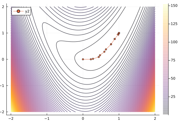
Here, NLPModels is used to access the function obj.

We can also use callbacks to exert more control over the algorithm. For instance, to implement a check on whether the objective value is stalling, we can define the following callback:

fold = -Inf
cb = (nlp, solver, stats) -> begin
  global fold
  f = stats.objective
  if abs(f - fold) / (abs(f) + abs(fold) + 1e-8) < 1e-3
    stats.status = :user
  end
  fold = f
end

output = trunk(nlp, callback=cb, rtol=0.0, atol=0.0)
println(output)

Generic Execution stats
  status: user-requested stop
  objective value: 1.405115328770847e-20
  primal feasibility: 0.0
  dual feasibility: 1.4364101353965366e-10
  solution: [0.9999999999573873  0.9999999999104003  0.999999999934689  0.9999999998670257 ⋯ 0.999999999938523]
  iterations: 18
  elapsed time: 0.004938840866088867

Above, we set the status of the algorithm to :user, so that it stops with a user-request stop flag.

---

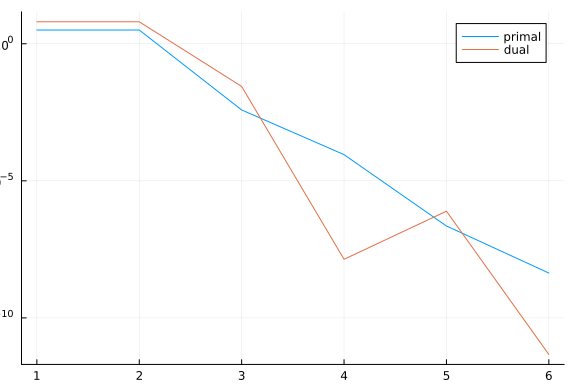
trunk is not the only solver that accepts callbacks. All solvers in JSOSolvers, as well as percival and dci from Percival.jl and DCISolver.jl do as well. Here is an example:

using Percival

@NLconstraint(model, [i=1:N], x[2i]^2 + x[2i-1]^2 <= 1.0)
nlp = MathOptNLPModel(model)

primal_history = Float64[]
dual_history = Float64[]
cb = (nlp, solver, output) -> begin
  push!(primal_history, output.primal_feas)
  push!(dual_history, output.dual_feas)
end
output = percival(nlp, callback=cb)

plt = plot()
plot!(plt, primal_history, lab="primal", yaxis=:log)
plot!(plt, dual_history, lab="dual")