by Abel S. Siqueira and Dominique Orban


In this tutorial we illustrate the main uses of SolverBenchmark.
First, let's create fake data. It is imperative that the data for each solver be stored in DataFrames, and the collection of different solver must be stored in a dictionary of Symbol to DataFrame.
In our examples we'll use the following data.
using DataFrames, Printf, Random

Random.seed!(0)

n = 10
names = [:alpha, :beta, :gamma]
stats = Dict(name => DataFrame(:id => 1:n,
         :name => [@sprintf("prob%03d", i) for i = 1:n],
         :status => map(x -> x < 0.75 ? :first_order : :failure, rand(n)),
         :f => randn(n),
         :t => 1e-3 .+ rand(n) * 1000,
         :iter => rand(10:10:100, n),
         :irrelevant => randn(n)) for name in names)
Dict{Symbol, DataFrames.DataFrame} with 3 entries:
  :alpha => 10×7 DataFrame…
  :beta  => 10×7 DataFrame…
  :gamma => 10×7 DataFrame…
The data consists of a (fake) run of three solvers alpha, beta and gamma. Each solver has a column id, which is necessary for joining the solvers (names can be repeated), and columns name, status, f, t and iter corresponding to problem results. There is also a column irrelevant with extra information that will not be used to produce our benchmarks.
Here are the statistics of solver alpha:
stats[:alpha]
10×7 DataFrame
 Row │ id     name     status       f           t        iter   irrelevant
     │ Int64  String   Symbol       Float64     Float64  Int64  Float64
─────┼─────────────────────────────────────────────────────────────────────
   1 │     1  prob001  first_order  -0.0242466  677.623     60  -1.15534
   2 │     2  prob002  first_order  -0.384201   645.643     90  -1.35454
   3 │     3  prob003  failure       0.578679   634.037     50  -0.117157
   4 │     4  prob004  failure       1.46765    559.585     70   1.15241
   5 │     5  prob005  first_order  -1.76643    567.557     10  -0.0381476
   6 │     6  prob006  first_order   0.608755   343.518     20  -1.00298
   7 │     7  prob007  first_order  -0.140199   426.141     10  -0.79729
   8 │     8  prob008  failure       0.835692   621.998     20   0.744854
   9 │     9  prob009  first_order  -0.929152   148.249     40   0.795775
  10 │    10  prob010  first_order   0.0788921  230.955     30  -0.839227
The first thing we may want to do is produce a table for each solver. Notice that the solver result is already a DataFrame, so there are a few options available in other packages, as well as simply printing the DataFrame. Our concern here is two-fold: producing publication-ready LaTeX tables, and web-ready markdown tables.
The simplest use is pretty_stats(io, dataframe). By default, io is stdout:
using SolverBenchmark

pretty_stats(stats[:alpha])
┌────────┬─────────┬─────────────┬───────────┬───────────┬────────┬────────────┐
│     id │    name │      status │         f │         t │   iter │ irrelevant │
├────────┼─────────┼─────────────┼───────────┼───────────┼────────┼────────────┤
│      1 │ prob001 │ first_order │ -2.42e-02 │  6.78e+02 │     60 │  -1.16e+00 │
│      2 │ prob002 │ first_order │ -3.84e-01 │  6.46e+02 │     90 │  -1.35e+00 │
│      3 │ prob003 │     failure │  5.79e-01 │  6.34e+02 │     50 │  -1.17e-01 │
│      4 │ prob004 │     failure │  1.47e+00 │  5.60e+02 │     70 │   1.15e+00 │
│      5 │ prob005 │ first_order │ -1.77e+00 │  5.68e+02 │     10 │  -3.81e-02 │
│      6 │ prob006 │ first_order │  6.09e-01 │  3.44e+02 │     20 │  -1.00e+00 │
│      7 │ prob007 │ first_order │ -1.40e-01 │  4.26e+02 │     10 │  -7.97e-01 │
│      8 │ prob008 │     failure │  8.36e-01 │  6.22e+02 │     20 │   7.45e-01 │
│      9 │ prob009 │ first_order │ -9.29e-01 │  1.48e+02 │     40 │   7.96e-01 │
│     10 │ prob010 │ first_order │  7.89e-02 │  2.31e+02 │     30 │  -8.39e-01 │
└────────┴─────────┴─────────────┴───────────┴───────────┴────────┴────────────┘
Printing is LaTeX format is achieved with pretty_latex_stats:
pretty_latex_stats(stats[:alpha])
\begin{longtable}{rrrrrrr}
  \hline
  id & name & status & f & t & iter & irrelevant \\\hline
  \endfirsthead
  \hline
  id & name & status & f & t & iter & irrelevant \\\hline
  \endhead
  \hline
  \multicolumn{7}{r}{{\bfseries Continued on next page}}\\
  \hline
  \endfoot
  \endlastfoot
  \(     1\) & prob001 & first\_order & \(-2.42\)e\(-02\) & \( 6.78\)e\(+02\) & \(    60\) & \(-1.16\)e\(+00\) \\
  \(     2\) & prob002 & first\_order & \(-3.84\)e\(-01\) & \( 6.46\)e\(+02\) & \(    90\) & \(-1.35\)e\(+00\) \\
  \(     3\) & prob003 & failure & \( 5.79\)e\(-01\) & \( 6.34\)e\(+02\) & \(    50\) & \(-1.17\)e\(-01\) \\
  \(     4\) & prob004 & failure & \( 1.47\)e\(+00\) & \( 5.60\)e\(+02\) & \(    70\) & \( 1.15\)e\(+00\) \\
  \(     5\) & prob005 & first\_order & \(-1.77\)e\(+00\) & \( 5.68\)e\(+02\) & \(    10\) & \(-3.81\)e\(-02\) \\
  \(     6\) & prob006 & first\_order & \( 6.09\)e\(-01\) & \( 3.44\)e\(+02\) & \(    20\) & \(-1.00\)e\(+00\) \\
  \(     7\) & prob007 & first\_order & \(-1.40\)e\(-01\) & \( 4.26\)e\(+02\) & \(    10\) & \(-7.97\)e\(-01\) \\
  \(     8\) & prob008 & failure & \( 8.36\)e\(-01\) & \( 6.22\)e\(+02\) & \(    20\) & \( 7.45\)e\(-01\) \\
  \(     9\) & prob009 & first\_order & \(-9.29\)e\(-01\) & \( 1.48\)e\(+02\) & \(    40\) & \( 7.96\)e\(-01\) \\
  \(    10\) & prob010 & first\_order & \( 7.89\)e\(-02\) & \( 2.31\)e\(+02\) & \(    30\) & \(-8.39\)e\(-01\) \\\hline
\end{longtable}
If only a subset of columns should be printed, the DataFrame should be indexed accordingly:
df = stats[:alpha]
pretty_stats(df[!, [:name, :f, :t]])
┌─────────┬───────────┬───────────┐
│    name │         f │         t │
├─────────┼───────────┼───────────┤
│ prob001 │ -2.42e-02 │  6.78e+02 │
│ prob002 │ -3.84e-01 │  6.46e+02 │
│ prob003 │  5.79e-01 │  6.34e+02 │
│ prob004 │  1.47e+00 │  5.60e+02 │
│ prob005 │ -1.77e+00 │  5.68e+02 │
│ prob006 │  6.09e-01 │  3.44e+02 │
│ prob007 │ -1.40e-01 │  4.26e+02 │
│ prob008 │  8.36e-01 │  6.22e+02 │
│ prob009 │ -9.29e-01 │  1.48e+02 │
│ prob010 │  7.89e-02 │  2.31e+02 │
└─────────┴───────────┴───────────┘
Markdown tables may be generated by supplying the PrettyTables tf keyword argument to specify the table format:
pretty_stats(df[!, [:name, :f, :t]], tf=tf_markdown)
|    name |         f |         t |
|---------|-----------|-----------|
| prob001 | -2.42e-02 |  6.78e+02 |
| prob002 | -3.84e-01 |  6.46e+02 |
| prob003 |  5.79e-01 |  6.34e+02 |
| prob004 |  1.47e+00 |  5.60e+02 |
| prob005 | -1.77e+00 |  5.68e+02 |
| prob006 |  6.09e-01 |  3.44e+02 |
| prob007 | -1.40e-01 |  4.26e+02 |
| prob008 |  8.36e-01 |  6.22e+02 |
| prob009 | -9.29e-01 |  1.48e+02 |
| prob010 |  7.89e-02 |  2.31e+02 |
All values of tf accepted by PrettyTables may be used in SolverBenchmark.
The fmt_override option overrides the formatting of a specific column. The argument should be a dictionary of Symbol to format strings, where the format string will be applied to each element of the column.
The hdr_override changes the column headers.
fmt_override = Dict(:f => "%+10.3e",
                    :t => "%08.2f")
hdr_override = Dict(:name => "Name", :f => "f(x)", :t => "Time")
pretty_stats(stdout,
             df[!, [:name, :f, :t]],
             col_formatters = fmt_override,
             hdr_override = hdr_override)
┌─────────┬────────────┬──────────┐
│    Name │       f(x) │     Time │
├─────────┼────────────┼──────────┤
│ prob001 │ -2.425e-02 │ 00677.62 │
│ prob002 │ -3.842e-01 │ 00645.64 │
│ prob003 │ +5.787e-01 │ 00634.04 │
│ prob004 │ +1.468e+00 │ 00559.59 │
│ prob005 │ -1.766e+00 │ 00567.56 │
│ prob006 │ +6.088e-01 │ 00343.52 │
│ prob007 │ -1.402e-01 │ 00426.14 │
│ prob008 │ +8.357e-01 │ 00622.00 │
│ prob009 │ -9.292e-01 │ 00148.25 │
│ prob010 │ +7.889e-02 │ 00230.96 │
└─────────┴────────────┴──────────┘
While col_formatters is for simple format strings, the PrettyTables API lets us define more elaborate formatters in the form of functions:
fmt_override = Dict(:f => "%+10.3e",
                    :t => "%08.2f")
hdr_override = Dict(:name => "Name", :f => "f(x)", :t => "Time")
pretty_stats(df[!, [:name, :f, :t]],
             col_formatters = fmt_override,
             hdr_override = hdr_override,
             formatters = (v, i, j) -> begin
               if j == 3  # t is the 3rd column
                 vi = floor(Int, v)
                 minutes = div(vi, 60)
                 seconds = vi % 60
                 micros = round(Int, 1e6 * (v - vi))
                 @sprintf("%2dm %02ds %06dμs", minutes, seconds, micros)
               else
                 v
               end
             end)
┌─────────┬────────────┬──────────────────┐
│    Name │       f(x) │             Time │
├─────────┼────────────┼──────────────────┤
│ prob001 │ -2.425e-02 │ 11m 17s 623091μs │
│ prob002 │ -3.842e-01 │ 10m 45s 642602μs │
│ prob003 │ +5.787e-01 │ 10m 34s 037248μs │
│ prob004 │ +1.468e+00 │  9m 19s 585367μs │
│ prob005 │ -1.766e+00 │  9m 27s 556767μs │
│ prob006 │ +6.088e-01 │  5m 43s 518002μs │
│ prob007 │ -1.402e-01 │  7m 06s 141220μs │
│ prob008 │ +8.357e-01 │ 10m 21s 997591μs │
│ prob009 │ -9.292e-01 │  2m 28s 248989μs │
│ prob010 │ +7.889e-02 │  3m 50s 955096μs │
└─────────┴────────────┴──────────────────┘
See the PrettyTables.jl documentation for more information.
When using LaTeX format, the output must be understood by LaTeX. By default, numerical data in the table is wrapped in inline math environments. But those math environments would interfere with our formatting of the time. Thus we must first disable them for the time column using col_formatters, and then apply the PrettyTables formatter as above:
fmt_override = Dict(:f => "%+10.3e",
                    :t => "%08.2f")
hdr_override = Dict(:name => "Name", :f => "f(x)", :t => "Time")
pretty_latex_stats(
df[!, [:name, :status, :f, :t, :iter]],
col_formatters = Dict(:t => "%f"),  # disable default formatting of t
formatters = (v,i,j) -> begin
  if j == 4
    xi = floor(Int, v)
    minutes = div(xi, 60)
    seconds = xi % 60
    micros = round(Int, 1e6 * (v - xi))
    @sprintf("\\(%2d\\)m \\(%02d\\)s \\(%06d \\mu\\)s", minutes, seconds, micros)
  else
    v
  end
end
)
\begin{longtable}{rrrrr}
  \hline
  name & status & f & t & iter \\\hline
  \endfirsthead
  \hline
  name & status & f & t & iter \\\hline
  \endhead
  \hline
  \multicolumn{5}{r}{{\bfseries Continued on next page}}\\
  \hline
  \endfoot
  \endlastfoot
  prob001 & first\_order & \(-2.42\)e\(-02\) & \(11\)m \(17\)s \(623091 \mu\)s & \(    60\) \\
  prob002 & first\_order & \(-3.84\)e\(-01\) & \(10\)m \(45\)s \(642602 \mu\)s & \(    90\) \\
  prob003 & failure & \( 5.79\)e\(-01\) & \(10\)m \(34\)s \(037248 \mu\)s & \(    50\) \\
  prob004 & failure & \( 1.47\)e\(+00\) & \( 9\)m \(19\)s \(585367 \mu\)s & \(    70\) \\
  prob005 & first\_order & \(-1.77\)e\(+00\) & \( 9\)m \(27\)s \(556767 \mu\)s & \(    10\) \\
  prob006 & first\_order & \( 6.09\)e\(-01\) & \( 5\)m \(43\)s \(518002 \mu\)s & \(    20\) \\
  prob007 & first\_order & \(-1.40\)e\(-01\) & \( 7\)m \(06\)s \(141220 \mu\)s & \(    10\) \\
  prob008 & failure & \( 8.36\)e\(-01\) & \(10\)m \(21\)s \(997591 \mu\)s & \(    20\) \\
  prob009 & first\_order & \(-9.29\)e\(-01\) & \( 2\)m \(28\)s \(248989 \mu\)s & \(    40\) \\
  prob010 & first\_order & \( 7.89\)e\(-02\) & \( 3\)m \(50\)s \(955096 \mu\)s & \(    30\) \\\hline
\end{longtable}
In some occasions, instead of/in addition to showing individual results, we show a table with the result of multiple solvers.
df = join(stats, [:f, :t])
pretty_stats(stdout, df)
┌────────┬───────────┬───────────┬───────────┬───────────┬───────────┬───────────┐
│     id │   f_alpha │   t_alpha │    f_beta │    t_beta │   f_gamma │   t_gamma │
├────────┼───────────┼───────────┼───────────┼───────────┼───────────┼───────────┤
│      1 │ -2.42e-02 │  6.78e+02 │  5.90e-01 │  3.10e+01 │ -7.31e-01 │  5.23e+02 │
│      2 │ -3.84e-01 │  6.46e+02 │ -9.15e-01 │  1.94e+02 │ -1.38e+00 │  4.25e+02 │
│      3 │  5.79e-01 │  6.34e+02 │ -2.14e+00 │  5.16e+02 │  1.90e+00 │  2.48e+02 │
│      4 │  1.47e+00 │  5.60e+02 │  4.86e-01 │  7.12e+02 │  4.77e-01 │  8.39e+02 │
│      5 │ -1.77e+00 │  5.68e+02 │ -3.67e-01 │  1.17e+02 │  3.74e-01 │  3.24e+02 │
│      6 │  6.09e-01 │  3.44e+02 │ -1.44e+00 │  4.79e+02 │  1.36e+00 │  1.62e+02 │
│      7 │ -1.40e-01 │  4.26e+02 │  1.23e-01 │  6.62e+02 │  8.25e-04 │  8.83e+02 │
│      8 │  8.36e-01 │  6.22e+02 │  2.63e-01 │  3.84e+02 │ -2.04e+00 │  2.83e+02 │
│      9 │ -9.29e-01 │  1.48e+02 │  1.41e+00 │  1.15e+02 │  8.89e-01 │  4.88e+02 │
│     10 │  7.89e-02 │  2.31e+02 │ -1.89e+00 │  9.90e+02 │ -3.92e-01 │  3.70e+02 │
└────────┴───────────┴───────────┴───────────┴───────────┴───────────┴───────────┘
The column :id is used as guide on where to join. In addition, we may have repeated columns between the solvers. We convery that information with argument invariant_cols.
df = join(stats, [:f, :t], invariant_cols=[:name])
pretty_stats(stdout, df)
┌────────┬─────────┬───────────┬───────────┬───────────┬───────────┬───────────┬───────────┐
│     id │    name │   f_alpha │   t_alpha │    f_beta │    t_beta │   f_gamma │   t_gamma │
├────────┼─────────┼───────────┼───────────┼───────────┼───────────┼───────────┼───────────┤
│      1 │ prob001 │ -2.42e-02 │  6.78e+02 │  5.90e-01 │  3.10e+01 │ -7.31e-01 │  5.23e+02 │
│      2 │ prob002 │ -3.84e-01 │  6.46e+02 │ -9.15e-01 │  1.94e+02 │ -1.38e+00 │  4.25e+02 │
│      3 │ prob003 │  5.79e-01 │  6.34e+02 │ -2.14e+00 │  5.16e+02 │  1.90e+00 │  2.48e+02 │
│      4 │ prob004 │  1.47e+00 │  5.60e+02 │  4.86e-01 │  7.12e+02 │  4.77e-01 │  8.39e+02 │
│      5 │ prob005 │ -1.77e+00 │  5.68e+02 │ -3.67e-01 │  1.17e+02 │  3.74e-01 │  3.24e+02 │
│      6 │ prob006 │  6.09e-01 │  3.44e+02 │ -1.44e+00 │  4.79e+02 │  1.36e+00 │  1.62e+02 │
│      7 │ prob007 │ -1.40e-01 │  4.26e+02 │  1.23e-01 │  6.62e+02 │  8.25e-04 │  8.83e+02 │
│      8 │ prob008 │  8.36e-01 │  6.22e+02 │  2.63e-01 │  3.84e+02 │ -2.04e+00 │  2.83e+02 │
│      9 │ prob009 │ -9.29e-01 │  1.48e+02 │  1.41e+00 │  1.15e+02 │  8.89e-01 │  4.88e+02 │
│     10 │ prob010 │  7.89e-02 │  2.31e+02 │ -1.89e+00 │  9.90e+02 │ -3.92e-01 │  3.70e+02 │
└────────┴─────────┴───────────┴───────────┴───────────┴───────────┴───────────┴───────────┘
join also accepts hdr_override for changing the column name before appending _solver.
hdr_override = Dict(:name => "Name", :f => "f(x)", :t => "Time")
df = join(stats, [:f, :t], invariant_cols=[:name], hdr_override=hdr_override)
pretty_stats(stdout, df)
┌────────┬─────────┬────────────┬────────────┬───────────┬───────────┬────────────┬────────────┐
│     id │    name │ f(x)_alpha │ Time_alpha │ f(x)_beta │ Time_beta │ f(x)_gamma │ Time_gamma │
├────────┼─────────┼────────────┼────────────┼───────────┼───────────┼────────────┼────────────┤
│      1 │ prob001 │  -2.42e-02 │   6.78e+02 │  5.90e-01 │  3.10e+01 │  -7.31e-01 │   5.23e+02 │
│      2 │ prob002 │  -3.84e-01 │   6.46e+02 │ -9.15e-01 │  1.94e+02 │  -1.38e+00 │   4.25e+02 │
│      3 │ prob003 │   5.79e-01 │   6.34e+02 │ -2.14e+00 │  5.16e+02 │   1.90e+00 │   2.48e+02 │
│      4 │ prob004 │   1.47e+00 │   5.60e+02 │  4.86e-01 │  7.12e+02 │   4.77e-01 │   8.39e+02 │
│      5 │ prob005 │  -1.77e+00 │   5.68e+02 │ -3.67e-01 │  1.17e+02 │   3.74e-01 │   3.24e+02 │
│      6 │ prob006 │   6.09e-01 │   3.44e+02 │ -1.44e+00 │  4.79e+02 │   1.36e+00 │   1.62e+02 │
│      7 │ prob007 │  -1.40e-01 │   4.26e+02 │  1.23e-01 │  6.62e+02 │   8.25e-04 │   8.83e+02 │
│      8 │ prob008 │   8.36e-01 │   6.22e+02 │  2.63e-01 │  3.84e+02 │  -2.04e+00 │   2.83e+02 │
│      9 │ prob009 │  -9.29e-01 │   1.48e+02 │  1.41e+00 │  1.15e+02 │   8.89e-01 │   4.88e+02 │
│     10 │ prob010 │   7.89e-02 │   2.31e+02 │ -1.89e+00 │  9.90e+02 │  -3.92e-01 │   3.70e+02 │
└────────┴─────────┴────────────┴────────────┴───────────┴───────────┴────────────┴────────────┘
hdr_override = Dict(:name => "Name", :f => "\\(f(x)\\)", :t => "Time")
df = join(stats, [:f, :t], invariant_cols=[:name], hdr_override=hdr_override)
pretty_latex_stats(df)
\begin{longtable}{rrrrrrrr}
  \hline
  id & name & \(f(x)\)\_alpha & Time\_alpha & \(f(x)\)\_beta & Time\_beta & \(f(x)\)\_gamma & Time\_gamma \\\hline
  \endfirsthead
  \hline
  id & name & \(f(x)\)\_alpha & Time\_alpha & \(f(x)\)\_beta & Time\_beta & \(f(x)\)\_gamma & Time\_gamma \\\hline
  \endhead
  \hline
  \multicolumn{8}{r}{{\bfseries Continued on next page}}\\
  \hline
  \endfoot
  \endlastfoot
  \(     1\) & prob001 & \(-2.42\)e\(-02\) & \( 6.78\)e\(+02\) & \( 5.90\)e\(-01\) & \( 3.10\)e\(+01\) & \(-7.31\)e\(-01\) & \( 5.23\)e\(+02\) \\
  \(     2\) & prob002 & \(-3.84\)e\(-01\) & \( 6.46\)e\(+02\) & \(-9.15\)e\(-01\) & \( 1.94\)e\(+02\) & \(-1.38\)e\(+00\) & \( 4.25\)e\(+02\) \\
  \(     3\) & prob003 & \( 5.79\)e\(-01\) & \( 6.34\)e\(+02\) & \(-2.14\)e\(+00\) & \( 5.16\)e\(+02\) & \( 1.90\)e\(+00\) & \( 2.48\)e\(+02\) \\
  \(     4\) & prob004 & \( 1.47\)e\(+00\) & \( 5.60\)e\(+02\) & \( 4.86\)e\(-01\) & \( 7.12\)e\(+02\) & \( 4.77\)e\(-01\) & \( 8.39\)e\(+02\) \\
  \(     5\) & prob005 & \(-1.77\)e\(+00\) & \( 5.68\)e\(+02\) & \(-3.67\)e\(-01\) & \( 1.17\)e\(+02\) & \( 3.74\)e\(-01\) & \( 3.24\)e\(+02\) \\
  \(     6\) & prob006 & \( 6.09\)e\(-01\) & \( 3.44\)e\(+02\) & \(-1.44\)e\(+00\) & \( 4.79\)e\(+02\) & \( 1.36\)e\(+00\) & \( 1.62\)e\(+02\) \\
  \(     7\) & prob007 & \(-1.40\)e\(-01\) & \( 4.26\)e\(+02\) & \( 1.23\)e\(-01\) & \( 6.62\)e\(+02\) & \( 8.25\)e\(-04\) & \( 8.83\)e\(+02\) \\
  \(     8\) & prob008 & \( 8.36\)e\(-01\) & \( 6.22\)e\(+02\) & \( 2.63\)e\(-01\) & \( 3.84\)e\(+02\) & \(-2.04\)e\(+00\) & \( 2.83\)e\(+02\) \\
  \(     9\) & prob009 & \(-9.29\)e\(-01\) & \( 1.48\)e\(+02\) & \( 1.41\)e\(+00\) & \( 1.15\)e\(+02\) & \( 8.89\)e\(-01\) & \( 4.88\)e\(+02\) \\
  \(    10\) & prob010 & \( 7.89\)e\(-02\) & \( 2.31\)e\(+02\) & \(-1.89\)e\(+00\) & \( 9.90\)e\(+02\) & \(-3.92\)e\(-01\) & \( 3.70\)e\(+02\) \\\hline
\end{longtable}
Performance profiles are a comparison tool developed by Dolan and Moré, 2002 that takes into account the relative performance of a solver and whether it has achieved convergence for each problem. SolverBenchmark.jl uses BenchmarkProfiles.jl for generating performance profiles from the dictionary of DataFrames.
The basic usage is performance_profile(stats, cost), where cost is a function applied to a DataFrame and returning a vector.
using Plots

p = performance_profile(stats, df -> df.t)
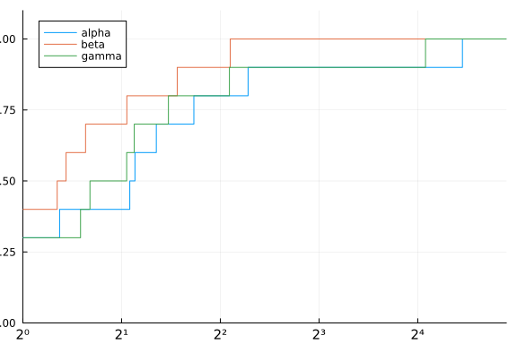
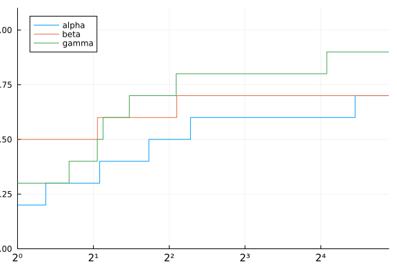
Notice that we used df -> df.t which corresponds to the column :t of the DataFrames. This does not take into account that the solvers have failed for a few problems (according to column :status). The next profile takes that into account.
cost(df) = (df.status .!= :first_order) * Inf + df.t
p = performance_profile(stats, cost)
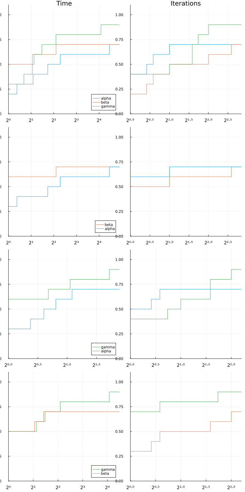
Another profile function is profile_solvers, which creates a wall of performance profiles, accepting multiple costs and doing 1 vs 1 comparisons in addition to the traditional performance profile.
solved(df) = (df.status .== :first_order)
costs = [df -> .!solved(df) * Inf + df.t, df -> .!solved(df) * Inf + df.iter]
costnames = ["Time", "Iterations"]
p = profile_solvers(stats, costs, costnames)
Here is a useful tutorial on how to use the benchmark with specific solver: Run a benchmark with OptimizationProblems The tutorial covers how to use the problems from OptimizationProblems to run a benchmark for unconstrained optimization.